

Abstract
Groundwater is critical to irrigated production in many arid and semiarid regions of the world. Groundwater that is low in quality presents limited value to farmers as an input to agricultural production. In this paper, we present findings from a survey of irrigator perceptions and irrigation water testing behavior targeted to producers in the Kansas portion of the High Plains Aquifer. Additionally, we estimate the value of an incremental increase in the quality of groundwater for agricultural irrigation using contingent valuation. We find that 30% of respondents have either “moderate” or “major” concern over the agricultural impacts of irrigation water quality. Additionally, 20% of respondents indicate that water quality has had either “moderate” or “major” impacts on their crop yields. Lastly, we find a median willingness to pay of US$39 well–1 for an incremental increase in irrigation water quality, as measured by reduced salt content.
Introduction
Agricultural intensification is often cited as a fundamental component to improving global food security and meeting growing demand for fiber and fuels (Tilman 1999). Intensification of agriculture is typified by use of high-yield crop varieties, chemical fertilizers, irrigation, and pesticides. As a result of decades of innovation to agricultural inputs, yields for important cereal crops are at all-time highs. Yields for each of barley (Hordeum vulgare L.), corn (Zea mays L.), rice (Oryza sativa L.), rye (Secale cereale L.), sorghum (Sorghum bicolor L.), and wheat (Triticum aestivum L.) are at least 100% above their mid-20th century averages (Schnitkey 2016). However, there are a number of diverse and detailed trade-offs between increased agricultural production and the environment. Some of the detrimental effects of agricultural practices on soil include erosion, declining soil organic matter, desertification, and salinization (Pimentel et al. 1995; Houk et al. 2006). Additionally, irrigated agriculture can both deplete finite sources of fresh water and deteriorate water systems through runoff and salts accumulation (Scanlon et al. 2007, 2012).
Over 56 million ac (22.6 million ha) of agricultural land is irrigated in the United States and approximately 60% of this total is irrigated from groundwater (Siebert et al. 2010). However, growing dependence of agricultural production on groundwater is causing rapid depletion of large aquifers. In the United States, depletion of the High Plains Aquifer (HPA) is particularly problematic. As groundwater is depleted, vertical depth to the water table will increase and a shallow saline water table may develop due to presence of naturally occurring salts in the aquifer, intrusion of saline surface water, or runoff of agricultural chemicals. Lands that are continually irrigated may therefore tend to develop increased salinity levels as fields are insufficiently drained and naturally occurring salts present in the parent aquifer material or chemical ions accumulate (Ghassemi et al. 1995). It is estimated that 25% to 30% of irrigated farmland in the United States experiences crop yield reductions stemming from high salinity soils, resulting in billions of dollars of lost potential crop production (Ghassemi et al. 1995).
In the central High Plains region, water quality degradation, as measured by total dissolved solids, has been attributed to agricultural irrigation (Scanlon et al. 2007). In southwest Kansas, interactions between the HPA and highly saline Arkansas River have raised concerns over the combined impacts of aquifer depletion and water quality degradation on future agricultural water demand in the region (Scanlon et al. 2012; Southwest Kansas Groundwater Management District Number 3 Board of Directors 2018). Well measurements of water in this region of Kansas have detected sulfate salinity concentrations above 1,500 mg L–1 (1,500 ppm) (Whittemore 2000; Whittemore et al. 2005), which is in the range where yield losses to corn, sorghum, and soybeans (Glycine max L.) can be detected (McFarland et al. 2014). Aquifer salinity is similarly a growing concern in other regions of Kansas (Lee 2019).
In this paper, we present findings from a recent survey of agricultural producers in the Kansas portion of the HPA on groundwater testing behavior and perceived impacts of groundwater quality on crop yields and planting decisions. Additionally, we estimate producer willingness to pay (WTP) for an incremental increase in the quality of their irrigation water, as measured by a reduction in electrical conductivity (EC) measurements. In total, we evaluate completed survey data from 637 producers operating in 24 different counties over the Kansas HPA. Data on the perceived impacts of irrigation water quality on agricultural outcomes and on WTP for improved groundwater quality can provide important information to producers, lenders, and policymakers considering investments in water and soil reclamation projects.
Based on the survey data, we find that one-third of respondents indicated either “moderate” or “major” concern over the agricultural impacts of water quality. By comparison, about one-half of respondents indicated either “moderate” or “major” concern over the agricultural impacts of water quantity, as measured by well yield. Additionally, about 20% of respondents indicated that water quality has had either “moderate” or “major” impacts on their crop yields. Finally, we estimate producer WTP for improved irrigation water quality using a contingent valuation question. We estimate a WTP ranging from US$26 well–1 to US$39 well–1 for an incremental improvement in the salt content of irrigation water.
Literature Review. In a survey of 136 agricultural producers in Kansas, Smith et al. (2007) found that 95% either “agreed” or “strongly agreed” that Kansas groundwater quality needed to be protected. At the same time, however, Smith et al. (2007) found that approximately half the respondents either “agreed” or “strongly agreed” that environmental legislation was often unfair to agricultural producers. Similarly, Pease and Bosch (1994) found that most producers express concern about water quality, but do not think government regulation on water quality should increase.
Many studies on water quality use contingent valuation to estimate WTP for quality changes due to a general absence of formal markets where water quality improvements can be bought and sold. Contingent valuation can be defined as a method to ascertain monetary value for goods and services not traded in a marketplace using data from surveys (Carson 2000). While previous studies have examined WTP for water quality, many of these studies are focused on residential drinking water rather than water for agricultural irrigation (Carson 2012; Kling et al. 2012; Johnston et al. 2017).
Looking specifically at irrigation water quality, Lichtenberg and Zimmerman (1999) used contingent valuation to estimate WTP of mid-Atlantic producers to reduce leaching of fertilizers into the water table. Lichtenberg and Zimmerman (1999) estimated a WTP ranging from US$17 ac–1 to US$35 ac–1 (US$42 ha–1 to US$87 ha–1) and that WTP was heterogeneous across farm sizes. When looking at different farm management techniques that affect water quality, Cooper (1997) estimated farmers’ willingness to accept for different practices within different regions of the United States. Cooper (1997) found that most farmers are willing to accept conservation tillage with little to no payment; however, farmers would need payments between US$14 and US$32 ac–1 (US$35 to US$79 ha–1) to increase adoption rates of integrated pest management, legume crediting, manure testing, and soil moisture testing.
With respect to WTP for irrigation water quantity, Knapp et al. (2018) used nonlinear programming to estimate producer WTP in the Arkansas Delta when water is scarce. Knapp et al. (2018) found that farmers are willing to pay about US$33 ac-ft–1 (US$0.03 m–3) for surface water, which is higher than groundwater pumping costs during times of water scarcity. In a study similar to this paper, Suter et al. (2019) estimate WTP of producers for an incremental increase in irrigation well yields (i.e., pumping rates). They estimate a WTP over the HPA of about US$77 well–1 for a 100 gallon per minute (gpm) (6 L s–1) increase in well yield.
WTP for agricultural improvements to water quality can also be found in residential sectors through reductions in loading of nonpoint source pollution. Hite et al. (2002) estimate a public WTP of about US$47 capita–1 to subsidize agricultural producers to adopt technological innovations that would result in reduced nonpoint source pollution of fresh water sources in Mississippi.
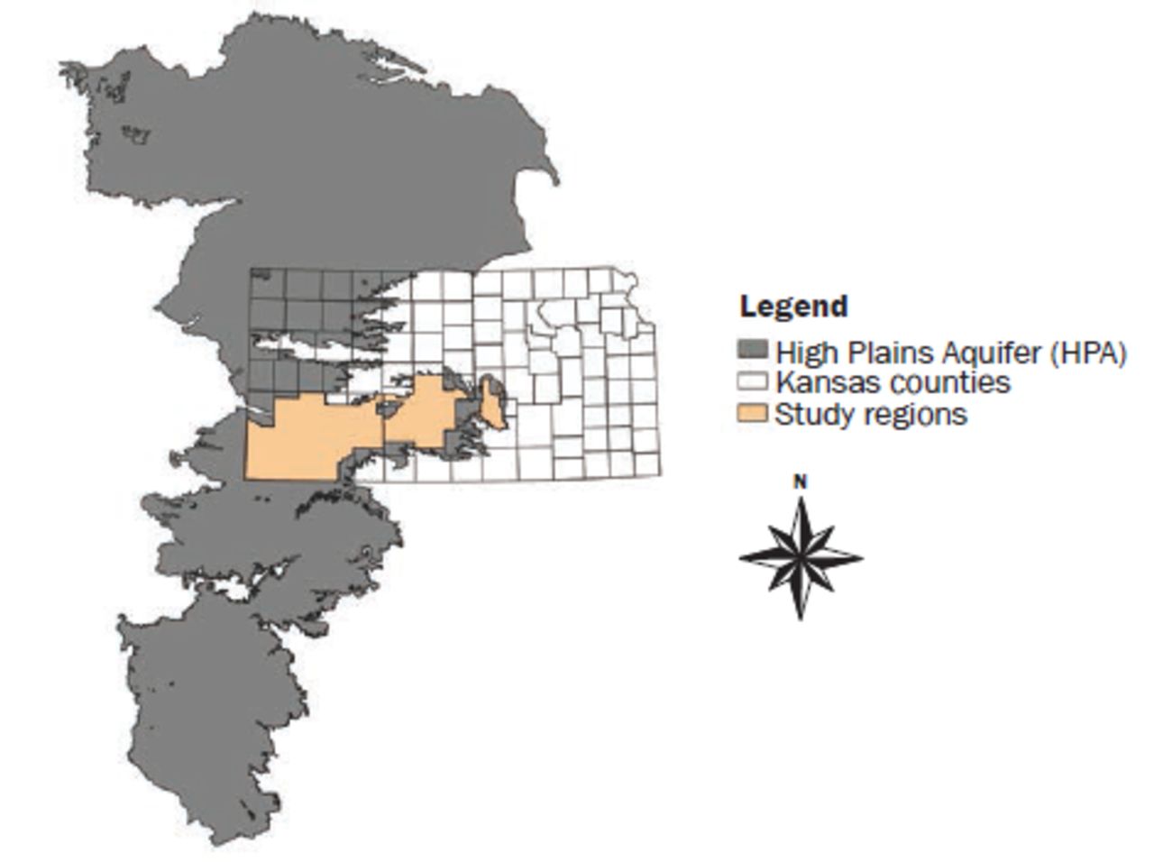
Background. The HPA underlies eight states, including Kansas, and spans from Texas to South Dakota (figure 1). In Kansas, irrigation from the aquifer is regularly applied to corn, sorghum, soybeans, alfalfa (Medicago sativa L.), and wheat (Lamm et al. 2012). Average annual extraction from the Kansas HPA is about 3.5 million ac-ft (4.3 billion m3) applied to 3 million irrigated acres (1.2 million ha) (Lanning-Rush 2016). Decades of pumping have led to water table declines across the Kansas HPA. It has been predicted that if depletion continues at current rates, irrigation will not be possible in 20 to 30 years (Haacker et al. 2016). In addition to water table declines, leaching of agricultural chemicals (Arias-Estévez et al. 2008) and nitrogen (N) through the soil profile (Letey and Vaughan 2013) affect water quality of the HPA. Rapid groundwater pumping has led to an upward movement in saline water, which increases the salinity of wells (Ma et al. 1997). In the southwest corner of the Kansas HPA, salinity has also increased due to highly saline Arkansas river water discharging into the aquifer (Whittemore 2000).

Study location in the High Plains Aquifer.
Irrigation water having high salt content injures crop germination and growth (Minhas et al. 2020). One solution to combat salinity is planting salt-tolerant crops. Crops typically planted in Kansas with a higher saline resiliency include soybeans and wheat. Reducing salinity of irrigation water and soils is also possible but poses some difficulty. Methods being explored include soil amendments (Mitchell et al. 2000), salt-tolerant cover crops (Gabriel et al. 2012), and irrigation practices that leave salt in the soil but below the root zone (Minhas et al. 2020). In principle, producers have an ongoing financial interest in lowering the salt content of water in the HPA in order to harvest crops that have a higher value per acre but lower salt tolerance (e.g., corn).
Materials and Methods
Fundamentally, contingent valuation exploits survey data to estimate monetary value for a nonmarketed good. The linkage between contingent valuation and WTP is established by utility theoretic models of consumer preference, which we do not detail here for the sake of succinctness. We refer interested readers to the expositions in Hanemann (1984), Bockstael and Freeman III (2005), and Carson and Hanemann (2005).
For the model of WTP to be empirically estimable, we assume that the WTP for each respondent i, which we term WTPi, can be expressed as a parametric function of observable and unobservable features that together influence the perceived net benefit of groundwater quality (i.e., reduced salinity). Let Xi denote demographic and farm characteristics for the ith respondent, ηi location-specific effects (i.e., Groundwater Management Districts [GMDs]) that might impact producer perceptions regarding irrigation and salinity, and ei denote the unobserved error term. Assuming that WTP is nonnegative and takes on an exponential form, we obtain equation 1:
 1
1
where β0 is a constant and β1 is a vector of parameters to be estimated.
Respondents will support the hypothetical program if their WTP is greater than the cost stated in the contingent valuation question, which we denote Ci. The probability of observing a “yes” to the hypothetical program is given by the following specification in equation 2:
 2
2
Following equation 2, the probability that the respondent supports the hypothetical program can be estimated using a log-logistic function as seen in equation 3. In particular, the logistic function estimates the probability of a respondent answering “yes” to the hypothetical program as a function of the log transformed stated bid amount [ln(Ci)], the demographic and farm characteristics (Xi), and location-specific effects (ηi):
 3
3
Coefficient estimates of β0, β1, and β2 for the model in equation 3 are obtained via maximum likelihood.
We choose to deploy a logit model over the alternative probit model due to the logit providing a marginally better fit and to increment off previous contingent valuation literature using the logit model (starting with Bishop and Heberlein 1979; Cameron 1988). A main advantage of using the log transform of the bid is that the mean WTP will be restricted to be nonnegative. Previous research has documented spatial heterogeneities in WTP for environmental improvements (Jørgensen et al. 2013; Czajkowski et al. 2017). In the context of irrigation in the Kansas HPA, WTP could be affected by region-specific characteristics such as hydrological features or rules regarding water use. To allow for this possibility, we include dummies for the three GMDs in our study area (i.e., ηi) and also cluster standard errors of the regression at the GMD level. The GMD-specific dummies will capture unobserved heterogeneity in responses that might systematically differ by GMD, while the clustered standard error allows for correlation in responses within GMDs.
To relate the model estimates to summary welfare measures, we report the median WTP (MWTP) following the recommendations by Hanemann (1984). In particular, the MWTP across all respondents is estimated from the log-logit regression model in equation 3 using the following specification in equation 4:
 4
4
where the “hat” notation denotes parameter estimates from the logit regression and σ is the vector of explanatory variables evaluated at their model sample averages.
Data Description. The project data are taken from a mail survey of agricultural producers in the Kansas portion of the HPA holding one or more rights to groundwater (figure 2).

Location of survey recipients and respondents.
Survey Design and Data. Under the Kansas Water Appropriation Act of 1945, any person seeking a right to use groundwater for agricultural production must apply to the Division of Water Resources of the Kansas Department of Agriculture for a permit. If the permit holder drills a well and puts the groundwater to beneficial use within the allowed window of time, then the water right is granted. Water rights are limited in the maximum annual quantities of water, maximum instantaneous pumping rates, and the locations from where the water is pumped and put to use (K.S.A. 82a-704c, K.S.A. 82a-708b).
Data for the analysis were collected from agricultural irrigators in the Kansas portion of the HPA using a mail survey (figures 1 and 2). To administer the survey, we obtained mailing addresses registered to all groundwater rights for agricultural irrigation in GMDs 2, 3, and 5 from the Division of Water Resources. In total, we obtained mailing address for 3,924 irrigators. We focus on GMDs 2, 3, and 5 because previous research has identified groundwater quality as a potential concern in this region (Whittemore 2000; Whittemore et al. 2005; Lee 2019). Figure 2 illustrates the groundwater well locations registered under the 3,924 irrigators included in the survey. The survey region covers 24 counties in Kansas (table 1).
Survey sample counties.
The goal of the survey was to obtain information about irrigation practices and attitudes toward irrigation water quality for agricultural producers. The survey contained questions pertaining to agricultural sales, producer demographics, farm size, planting and irrigation practices, history of testing the chemical quality of irrigation water, and perceived seriousness of irrigation water quality impacts on planting decisions and crop yield. The survey concluded with a contingent valuation question focused on salinity of irrigation water.
Advance postcards were mailed to all 3,924 irrigators on March 4, 2020. The advance postcards briefly informed recipients of the survey’s intention as a tool to collect information for academic research. The full survey was mailed on March 10 and 11, 2020. A follow-up postcard containing a brief reminder message was mailed to all 3,924 irrigators on March 23, 2020. Of the 3,924 irrigators in the mail survey sample, 308 had their surveys returned by the US Postal Service because the survey was not deliverable as addressed. Thus, we assume there were 3,616 surveys that were delivered as addressed using the contact information from the Division of Water Resources. There were 990 total surveys returned. Of this total, there were 117 returned surveys where the recipient did not answer any of the survey questions and 105 surveys where the recipient did not answer the contingent valuation question. Completed surveys were received from 768 irrigators, giving a 21.2% response rate (i.e., 768/3,616).
We limit the analysis to survey recipients indicating that they had one or more active irrigation wells on their farmland and at least some irrigated area composing their total farm area (103 observations dropped). We drop observations having more than 50 irrigation wells because they are likely to represent farming collectives (2 observations dropped). In an attempt to detect protest bids and insincere responses, we included the following statement, where recipients were asked to respond true or false: “A high salt content in irrigation water is good for crop growth.” Recipients who left the true/false blank or who answered true were excluded from the analysis (26 observations dropped).
In sum, we were left with 637 completed surveys. All 24 counties were represented in the 637 survey responses, with county-specific respondent shares ranging from 8% to 22% (figure 2, table 1).
Contingent Valuation Question. The final page of the survey packet contained a contingent valuation question, where respondents were presented with a hypothetical scenario that described an aquifer remediation project and were asked whether they supported the project at a stated cost per irrigation well. The contingent valuation question was designed to complement and build off of a previous survey focused on irrigation well capacity that was sent to producers in the Ogallala Aquifer portions of Kansas, Colorado, Nebraska, New Mexico, Oklahoma, and Texas in 2018 (Suter et al. 2019). In particular, the phrasing and hypothetical charge specified in the question was influenced by the contingent valuation question of Suter et al. (2019) due to geographic overlap in the survey sample (i.e., some producers may have received both surveys). The contingent valuation question read:
The High Plains Aquifer underlies portions of northwestern, western, southwestern, and southcentral Kansas. The majority of water from the High Plains Aquifer in Kansas is used for agricultural production, serving as an important input to producing valuable crops such as corn and soybean. Groundwater in areas across the Kansas High Plains Aquifer is experiencing deteriorated water quality such as high concentrations of chloride (Cl–) and sulfate salts that could result in lowered crop productivity, lowered crop yield, and degraded topsoil. Electrical conductivity (EC) is used as a general measure of the chemical quality of irrigation water. Low EC measurement is generally desirable for agricultural irrigation use because it indicates a low salt content of the water.
Suppose that, to address groundwater quality, the state of Kansas is considering a one-time charge of US$[A] per irrigation well that would be charged to all producers that use groundwater for agricultural irrigation in your area. This charge would be included in your 2020 local property taxes and would finance an aquifer remediation program, leading to an average of [B] mmho/cm reduction in the EC measurement of irrigation groundwater in your area within 2 years (i.e., a lower salt content).
The one-time charge was taken at random from one of five possible values, A = (250; 1,000; 2,000; 3,000; 5,000). The reduction in the EC measurement of irrigation water was taken at random from one of two possible values, B = (1, 3). The bid amounts were selected due to potential familiarity of respondents with the Suter et al. (2019) survey and as a means to compare WTP for irrigation water quality improvements against recent literature estimates of WTP for groundwater quantity (e.g., Knapp et al. 2018; Suter et al. 2019). Ten different contingent valuation questions were created based on the five potential one-time charge values and two potential EC measurement improvement values. The ten different versions were assigned to recipients at random by county, such that each of the 24 counties in the study region had an approximately equal distribution of the contingent valuation question. Provision of the environmental service that respondents were bidding on (i.e., lower salt content) was limited in its geographic and temporal scope, consistent with the recommendations set out by Haab and McConnell (2002). The vehicle for payment of the service was made clear to respondents (i.e., included in 2020 property taxes).
Recipients were also provided a brief definition of EC, including some background information provided by the USDA Natural Resources Conservation Service (1997) so that the environmental service described in the contingent valuation question could be interpreted in terms commonly understood by agricultural producers. The statement is presented in figure 3.

Background information provided by the USDA Natural Resources Conservation Service (1997).
Following the description of the hypothetical program, recipients were asked a dichotomous choice question indicating whether or not they supported the program. We opted for a single bounded dichotomous choice format for two reasons. First, Johnston et al. (2017) argue that dichotomous choice formats ensure incentive compatibility in contingent valuation applications. Second, the single bounded format provides a shorter, more straightforward choice setup to the respondent in a mailed survey. Overall, the contingent valuation method used was consistent with standard practices set forth in the nonmarket valuation literature (Haab and McConnell 2002; Johnston et al. 2017).
Irrigator and Farm Characteristics. The survey contained questions on irrigator and farm characteristics that might impact the perceived benefits of irrigation water quality improvements (tables 2 and 3). We briefly summarize these characteristics in this section. Over 40% of respondents reported that their annual revenues from agricultural sales exceeded US$500,000. About two-thirds of respondents indicated that 80% to 100% of their total agricultural sales derive from crop commodities (as opposed to e.g., livestock). By comparison, the 2017 USDA Agricultural Census indicates an average market value of agricultural products sold of US$1.3 million farm–1 in Kansas for irrigated operations. The proportion of total farm area that is irrigated was approximately uniform across respondents, with 22% of respondents reporting that less than 25% of their farm area was irrigated and 22% of respondents reporting that more than 75% of their farm area was irrigated. Half of respondents indicated they owned at least 75% of the irrigated area in operation. Only 8% of respondents reported they were tenant operators for irrigated land, which we further discuss in the results section. We hypothesize that ownership of irrigated land will be positively correlated with support for the program because aquifer characteristics are capitalized into land values (Sampson et al. 2019).
Farm and demographic summary statistics.
Full description for categorical variables.
Half of respondents possessed a college degree or higher. Two-thirds of respondents indicated that their main residence is on the farm. The average respondent age was about 65 years. By comparison, the average age of farmers in Kansas according to the 2017 USDA Agricultural Census was 58 years. We hypothesize that younger irrigators are more willing to support the remediation program because they would benefit for a longer time span from the improved water quality. Both education and on-farm residence are hypothesized to be positively correlated with support for the remediation program.
We obtain a count of active points of diversion (i.e., irrigation wells) from the Water Information Management and Analysis System (WIMAS) operated by the Division of Water Resources. The average number of active wells per respondent was 3.80, with a minimum of 1 and a maximum of 35. Over three-quarters of respondents indicated their average well yield was between 400 and 1,000 gpm (25 to 63 L s–1). Approximately 18% of respondents indicated well yield below 400 gpm. The modal irrigation application rate was between 1 and 2 ac-ft ac–1 (3,048 to 6,096 m3 ha–1), which is generally consistent with corn water demand in Kansas (Rogers et al. 2015). It is unclear ex ante how the number of wells will impact support for the remediation program. Total cost for the program increases linearly in the number of wells while the returns to scale with respect to well number is unclear.
Perceptions toward Groundwater Chemical Quality. Approximately one-third of respondents indicated they had either “moderate concern” or “major concern” about irrigation water quality in their area (table 4). By comparison, about half of respondents had “moderate concern” or “major concern” about irrigation well yields in their area. We further examined concerns over water quality by asking irrigators to indicate the impact that irrigation water quality has had on their crop yield and crop mix decisions. Over 20% of respondents indicated that irrigation water quality has had “moderate impact” or “major impact” on their yields. About 15% of respondents indicated that irrigation water quality has had “moderate impact” or “major impact” on their cropping decisions.
Irrigation water quality testing and irrigator perceptions.
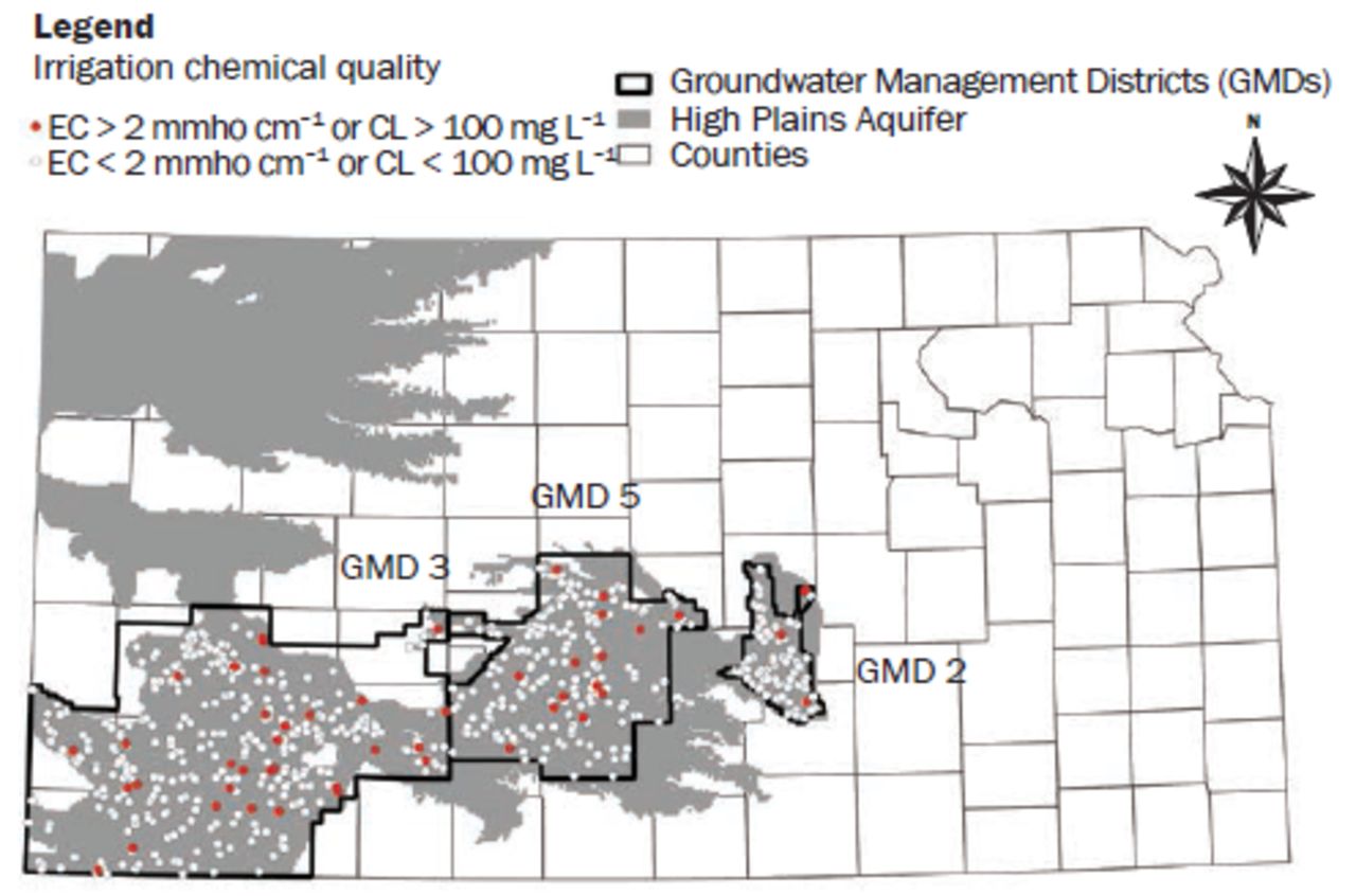
Despite the water quality concerns, nearly half of respondents indicated they have never tested the chemical quality of their irrigation water. In fact, only about one-third of respondents have tested their water in the last five years. For those who did know the EC measurement of their water, about one-quarter of respondents indicated a measurement of 2 mmho cm–1 (1 mmho cm–1 = 1 mS cm–1) or greater (figure 4, table 4). Likewise, for those irrigators knowing the Cl– content of their water, about one-fifth indicated a measurement of 100 mg L–1 (100 ppm) or greater (figure 4, table 4). For context, the Natural Resources Conservation Service (NRCS) advises severe crop water availability problems starting at 3 mmho cm–1 for salinity and moderate plant toxicity starting at 100 mg L–1 for Cl– (USDA NRCS 1997).

Location of respondents who have tested their water quality and locations indicating irrigation water measurements of electrical conductivity (EC) > 2 mmho cm–1 or chloride (Cl) > 100 mg L–1.
Results and Discussion
Willingness to Pay Analysis. In this section we present results from estimating equation 3 using the survey response data. In estimating equation 3, we did not include all variables from table 2 due to concerns with model efficiency and overfitting the model with factor variables. The variables included in the vector Xi are respondent age, off-farm residence, education, number of irrigation wells, proportion of farm that is irrigated, proportion of irrigated area that is owned, and an indicator for whether the respondent reported EC measures greater than 2 mmho cm–1.
Figure 5 provides a summary of the respondents that supported or did not support the hypothetical water quality remediation program. Support for the program is broken down by the one-time charge and the reduction in EC stated in the contingent valuation question. The responses to the contingent valuation question follow economic intuition in that the proportion of respondents supporting the program declines as the one-time charge increases. In particular, 17% of respondents support the program at the lowest bid amount (US$250 well–1) while only 4% of respondents support the program at the highest bid amount (US$5,000 well–1). For a fixed bid amount, there is generally greater support for the program when there is a greater reduction in EC. For example, at the lowest bid amount of US$250 well–1, 21% of respondents supported the program when there was a 3 mmho cm–1 reduction compared to just 11% of respondents when there was a 1 mmho cm–1 reduction. Likewise, at a US$1,000 well–1 bid amount, 19% of respondents supported the program when there was a 3 mmho cm–1 reduction compared to just 7% when there was a 1 mmho cm–1 reduction.
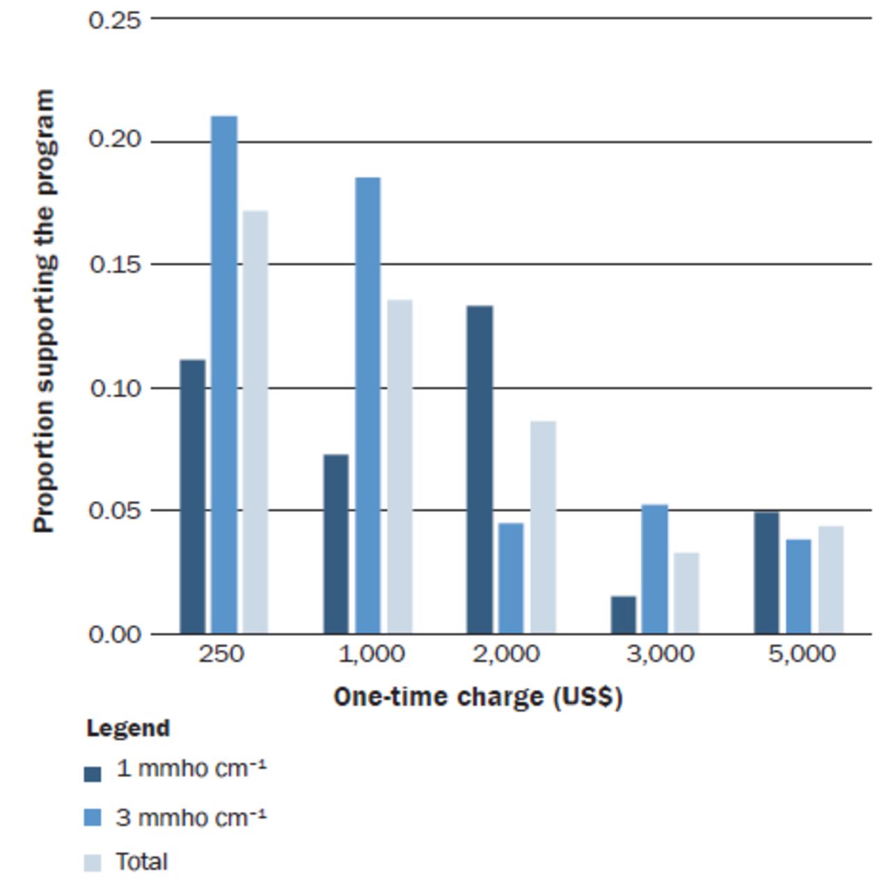
Proportion of respondents supporting the hypothetical water quality remediation program by bid amount and reduction in electrical conductivity (EC).
Table 5 reports the econometric results from estimating equation 3. Column 1 of table 5 reports estimates, which pools together data from all respondents. Column 2 of table 5 restricts the sample to respondents owning at least some of their irrigated area. Columns 3 and 4 of table 5 use the subsample from column 2 but divide the subsample according to respondents where the contingent valuation question indicated a 1 mmho cm–1 or 3 mmho cm–1 reduction in EC, respectively. We run separate regressions for the subsample in columns 3 and 4 as a way to check for heterogeneity in factors contributing to support of the program driven by the EC reduction without the need for extensive interaction terms in the regression specification.
Coefficient estimates of the regression.
Looking at column 1 of table 5, we find the coefficient on the logged bid is negative and statistically significant at 0.01. Thus, producers are responsive to the stated bid when determining support for the hypothetical program. As expected, as the stated bid value goes up, support for the hypothetical program goes down. The coefficient on the 3 mmho cm–1 reduction is positive but not statistically significant. The interpretation is that more respondents supported the hypothetical program for a 3 mmho cm–1 reduction in EC than a 1 mmho cm–1 reduction in EC, but the difference is not statistically significant. The indicator variable on known irrigation water EC measures greater than 2 mmho cm–1 is positive and statistically significant at 0.01, providing evidence that respondents having poorer water quality were more likely to support the hypothetical program.
Looking at the rest of the coefficients in column 1, we note that respondents having some college or a college degree were less likely to support the program than respondents having a high school diploma. One potential explanation is that respondents having college education might be relatively more willing to engage in technological innovations that might already be mitigating water quality impacts. Alternatively, the ability to attend college might correlate with larger or more profitable irrigated operations that might have better water quality on average. The coefficient on the number of wells is negative and statistically significant, indicating respondents with large-scale irrigation water use were less likely to support the program. One possible explanation is that producers perceived that the returns to improved irrigation water quality were decreasing in the total number of irrigation wells. Somewhat surprisingly, respondents who irrigated 25% to 50% or 50% to 75% of their farm area were less likely to support the program than respondents who only irrigated 0% to 25% of their farm area, though the effect is only weakly statistically significant. One possible interpretation is that the latter group coupled an increase in irrigation water quality with the potential to irrigate a greater share of their farm area.
Also surprisingly, respondents who did not own their irrigated area were more likely to support the hypothetical program. Evidence from comments written in by respondents suggests that a number of retired landowners forwarded the survey to their farmer tenants. To account for the possibility that tenants would support the program but ultimately never bear the cost of the program due to the payment vehicle being the property tax, we drop all observations where respondents indicate owning none of their irrigated area in columns 2 to 4. We generally find a pattern in coefficient estimates that is consistent with the results in column 1.
Using the coefficient estimates from the log-logistic regression in table 5, the MWTP for EC reduction per well can be estimated from equation 4. Coefficients for the GMD dummies were not statistically significant in columns 1, 2, and 4, so we do not estimate GMD-specific WTP for those specifications. Evaluating equation 4 at sample mean covariate values yields a MWTP of about US$39 well–1 using the full sample in column 1 and US$26 well–1 when restricting the subsample to owners only in column 2. Running separate regressions over the 1 mmho cm–1 and 3 mmho cm–1 subsamples reveals that the MWTP for a 3 mmho cm–1 reduction in EC is about US$47 well–1 (column 4) while the MWTP for a 1 mmho cm–1 reduction is not statistically different from zero (average effect, column 3). Additionally, looking at column 3, even though respondents in GMDs 3 and 5 were more likely to support the remediation program than respondents in GMD 2, the difference in MWTP for a 1 mmho cm–1 reduction across GMDs was not statistically significant.
Summary and Conclusions
While one-third of respondents indicated “moderate” or “major” concern over water quality, only 17% of respondents supported the water quality remediation program at the minimum bid amount. One interpretation of the gap between concern over water quality and support for the remediation program is producer reluctance to participate due to concern over more stringent future environmental regulation. For instance, Peterson et al. (2007) find that producers might have reluctance to engage in water quality trading due to concerns that future government regulation of agriculture would become more stringent.
Another possible explanation for the relatively low support for the hypothetical remediation program relates to the Coronavirus Disease 2019 (COVID-19) outbreak in the United States. Government shutdowns and shelter in place orders were not anticipated when the survey was first implemented in early March of 2020. Related to COVID-19 are trade restrictions, processing plant closures, and lowered oil prices, which in turn affect demand for ethanol feedstocks (e.g., corn). These impacts are likely to affect producer incomes and solvency, which might affect WTP for environmental amenities such as groundwater quality (Flores and Carson 1997; Hökby and Söderqvist 2003). Forward-looking respondents might have anticipated lowered 2020 farm incomes and thus a reticence to accept higher 2020 property tax through the remediation program.
Another potential interpretation relates to distributional aspects of the hypothetical aquifer remediation program. Numerous respondents wrote side-notes in the survey that irrigation water quality is not a homogeneous problem across the Kansas HPA. This evidence is consistent with previous studies documenting spatial heterogeneity in WTP for environmental improvements (Jørgensen et al. 2013; Czajkowski et al. 2017). In short, respondents might not wish to bear remediation costs for a problem they themselves were not directly responsible for. For example, in addition to the naturally occurring salts in aquifer material, past and present industrial activities pose risk to groundwater used for drinking and agriculture (Osborn et al. 2011; Vidic et al. 2013). Similarly, some respondents noted they were not willing to support such a program unless there were formal mechanisms for collective action. However, collective action to manage groundwater is made difficult in theory because actions taken in one location can affect water availability and quality in surrounding locations (Ostrom 1990; Brozovic et al. 2010; Sampson and Sanchirico 2019).
In a similar survey of agricultural producers, Suter et al. (2019) estimate median WTP for an incremental increase in irrigation well capacity for irrigators over the HPA. They estimate a WTP of US$77 well–1 for the six states overlying the HPA. Thus, our median WTP estimate of US$26 well–1 to US$39 well–1 for an incremental reduction in EC is about half of the median WTP for an incremental increase in well capacity estimated in Suter et al. (2019). This is not entirely surprising given that a larger number of respondents in this survey were more concerned with well yields than water quality. Additionally, water availability has long been associated with depletion of the HPA (Scanlon et al. 2012) while the conjoint problem of water quality is more of an emerging empirical issue.
From a research perspective, spatially detailed data on the quality of irrigation water are difficult to obtain. Additionally, based on this survey, testing of groundwater for chemical quality is not exactly customary amongst producers. Roughly two-thirds of respondents indicated they had never tested the chemical quality of their irrigation water or that the most recent test was older than 10 years. Increased data collection on the chemical quality of groundwater will support empirical projects aimed at connecting producer behavior and outcomes to groundwater characteristics. Apart from survey methods, outreach programs and focus group studies bringing together operators, landowners, and groundwater managers are a source of information that could help identify priority areas for protection and to direct reclamation funds to where they will make the greatest impacts.
In retrospect, the upper end of the stated bid amounts in the contingent valuation question were arguably too large. For instance, a producer having 10 irrigation wells and receiving a stated bid amount of US$5,000 well–1 would need to be willing and financially capable to bear a US$50,000 one-time charge to their local property tax in order to support the remediation program. We note this proviso in hopes that it can inform future surveys and contingent valuation questions focused on water quality.
Acknowledgements
Funding support for this study was provided by the John and Della Hodler Fund.
- Received June 9, 2020.
- Revision received October 30, 2020.
- Accepted November 1, 2020.
- © 2021 by the Soil and Water Conservation Society
References
In this issue


Jump to section
Related Articles
Cited By...
- No citing articles found.